What’s going on inside a JPEG?

Android Software Developer
Email: huynhnguyennhatminh98@gmail.com
A typical image is represented as a matrix corresponding to the intensity of the pixels. Color images use different channels for each color component, such as red, green, and blue. Most digital cameras today come with multiple lenses, high performance, and can capture high-quality photos. The amount of data needed to store or display those photos can be huge. For example, a photo taken on the Pixel 6 Pro has about 12.5 megapixels (4080 x 3072 resolution). If each pixel uses 24-bit depth (8 bits per each RBG channel), then the whole image is about 37.6 MB in size, which is not a small number. This is where JPEG comes in handy.
In 1992, the Joint Photographic Experts Group (hence the name JPEG) creates a standard to compress graphics files enough to work on the average PC. They came up with the concept of lossy compression, which removed visual data that the human eye couldn't see and averaged out color variation. Despite the huge reduction in file size, the JPEG images still maintain reasonably high quality. A JPEG file supports up to 24-bit color (16.8 million colors in total) while staying relatively small, which is very convenient for storing and sending the image. Nowadays, JPEG files are the most widely used images on the Internet, computers, and mobile devices… In this article, we will take a look at what is going on inside a JPEG to understand how can they achieve such an effective compression.
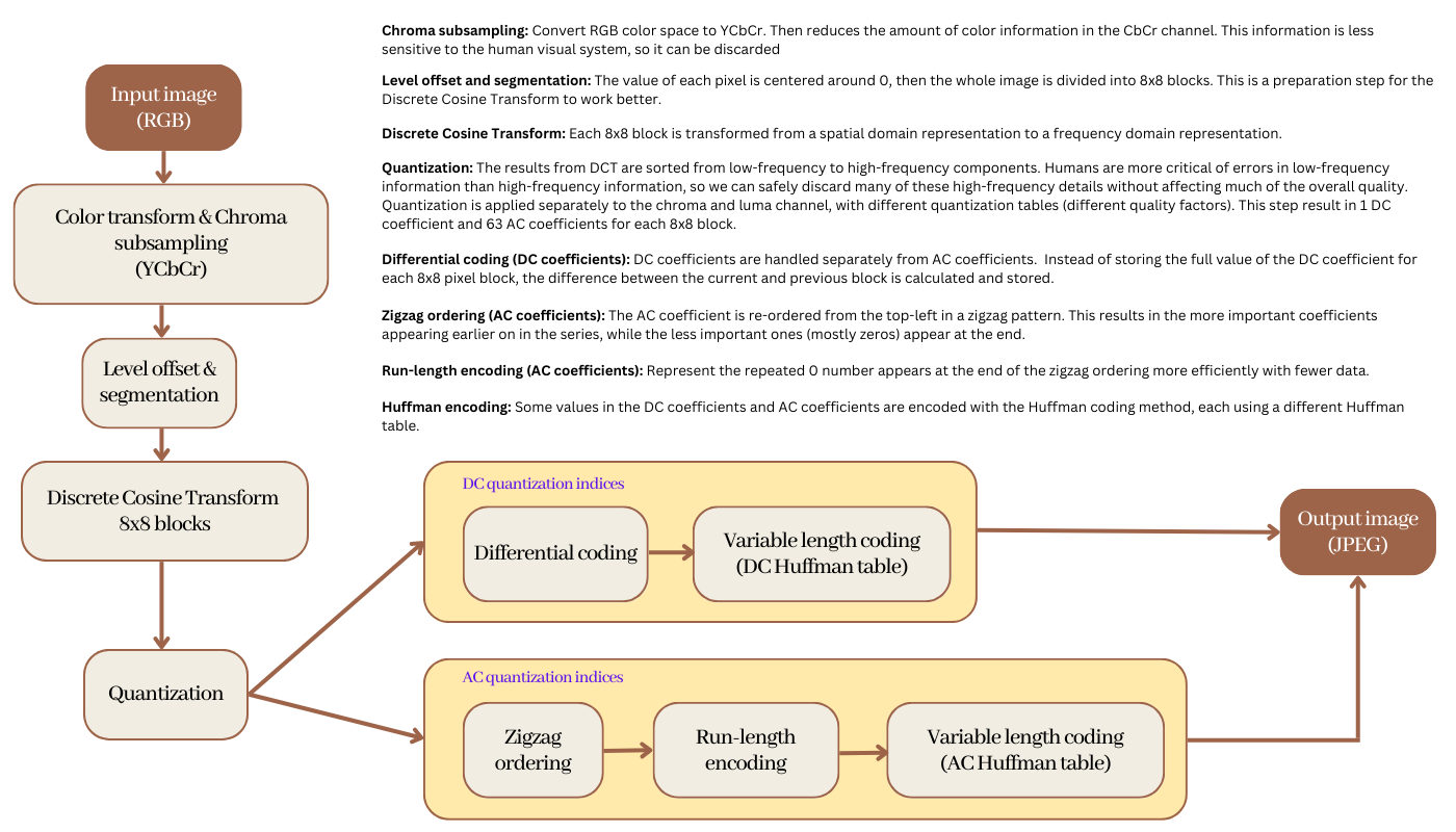
Chroma subsampling
In the human visual system, there are two kinds of specialized cells to absorb light and send visual signals to the brain. Rod cells, susceptible to light, transmit mostly black-and-white information to the brain. Whereas, cone cells are capable of detecting a wide spectrum of light photons and are responsible for color vision. There are over 120 million rod cells in each eye, compared to just 6 million cone cells. That means the human eye is more sensitive in detecting differences in luminance (brightness) than chrominance (color intensity) information.
The more color information that is required to represent an image, the more space it’ll take. So if we can discard some of the color information, we can make a smaller image. This technique is called chroma subsampling. It reduces the amount of color information in a source signal to allow more luminance data instead.
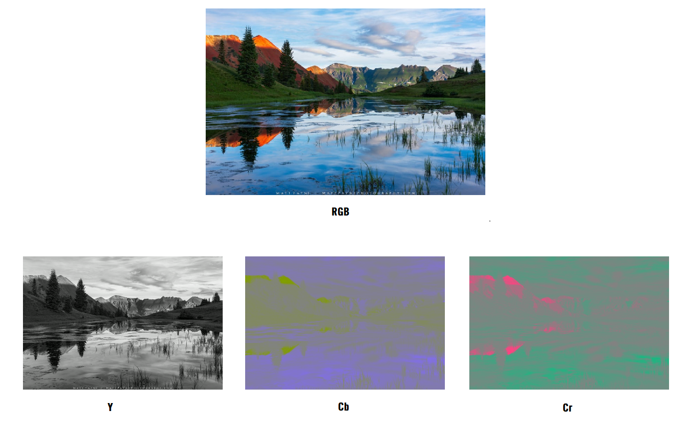
As you can see, when we split the luminance and chrominance of the photo, it becomes clear that the luminance channel is much more important. The luma channel (the grayscale image - Y) is sufficient for a clear impression of the image. The chroma channels (Cb and Cr), on the other hand, are much less clear. This kind of color space is called YCbCr.
To discard the color, there are several commonly used subsampling ratios for JPEGs, including:
4:4:4 - no subsampling
4:2:2 - reduction by half in the horizontal direction (50% area reduction)
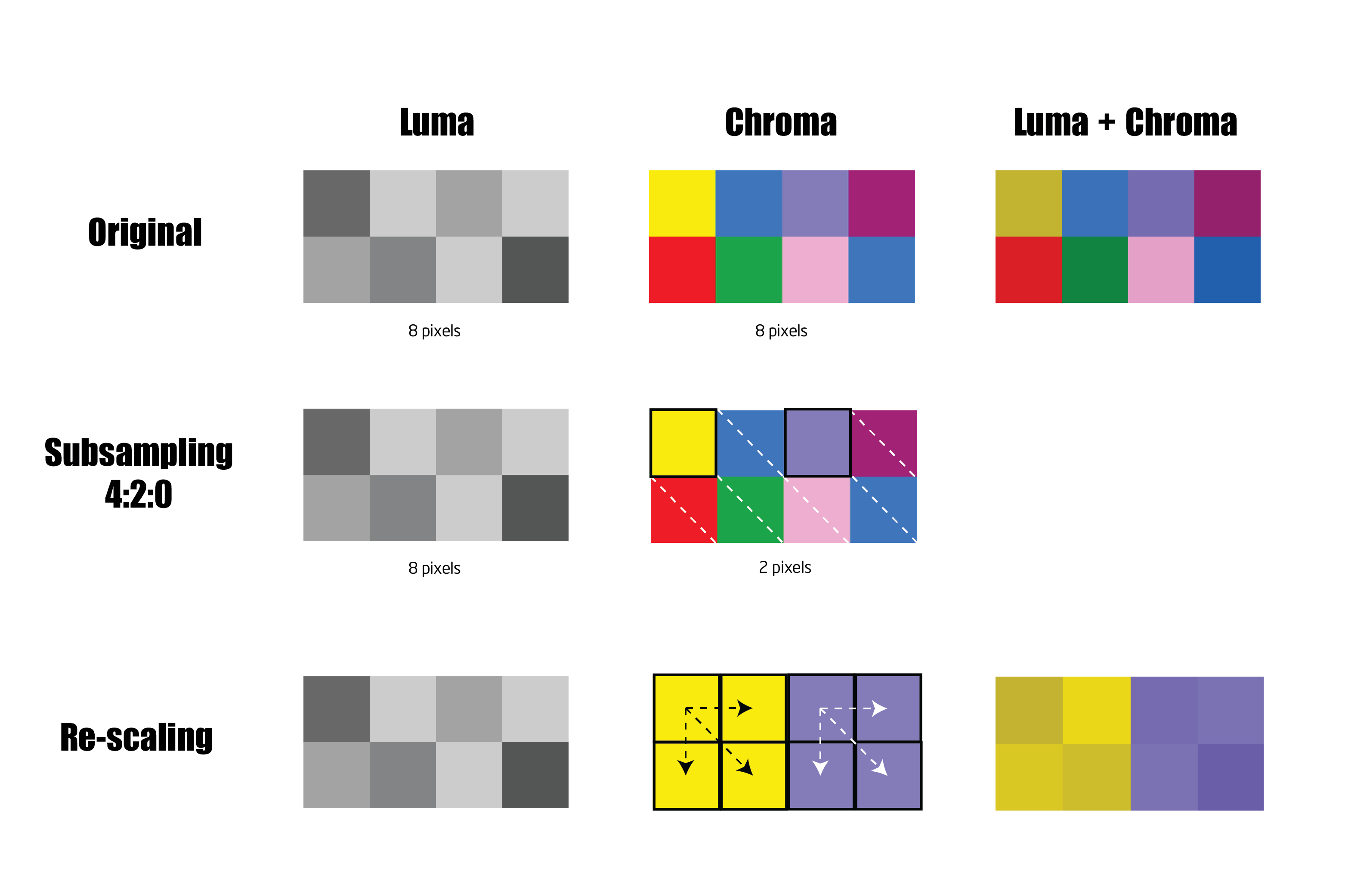
4:2:0 - reduction by half in both the horizontal and vertical directions (75% area reduction)

For example, with the chroma subsampling of 4:2:0, in each block of 4 pixels, we only keep 1 color and discard the other 3. That is a notable least data compared to the original.
Discrete Cosine Transform
This is perhaps the most confusing step in the process and is the most important one. We will explore this without going deep into the confusing mathematics and equations.
An image is often represented in the form of a 2D matrix, where each element of the matrix represents a pixel intensity. This, known as the spatial domain, serves the purpose of defining the exact pixels within an image. But the spatial domain is not suitable when we need to analyze and do calculations on the image. So to make things easier, we need to change it into something different.
One way to think about an image is to consider it as a “signal”. For instance, we can extract a specific row of pixels and plot it to represent some kind of signal wave.
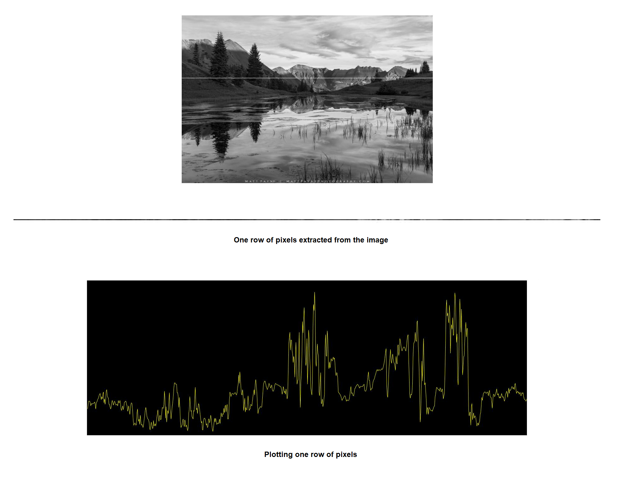
When displaying the image in this way, it is simple to find out the “frequency” of that image. Frequency is the rate of change of intensity values. Thus, a high-frequency image has intensity values that change quickly from one pixel to the next.
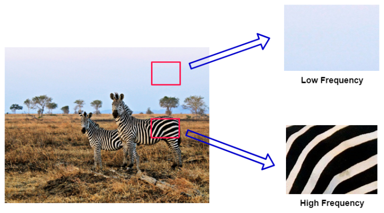
Images contain a wide range of frequencies. When the image is further away (or appears smaller), we rely more on the lower frequencies to grasp the gist of the image. From closer distances, we perceive high-frequency signals to figure out the detail. In general, humans are more critical of errors in low-frequency information than the high-frequency information. So we can discard many of these high-frequency details without decreasing the overall quality much.

Transforming images from the spatial to the frequency domain allows us to manipulate the higher-frequency data without affecting the low-frequency components. This is where we need the Discrete Cosine Transform (DCT). But before we dive into the DCT, we need to discuss something called the Fourier Transform.
Fourier Transform
In the early 1820s, Joseph Fourier, a French mathematician and physicist, figured out that any complex waveform can be broken into the sum of simple sinusoids (sine and cosine waves) of different amplitudes and frequencies.
That sounds nice, but why do we even care about that?
Well, complex signals made from the sum of sine waves are all around us. In fact, all signals in the real world can be represented as the sum of sine waves. The Fourier transform gives us insight into what sine wave frequencies make up a signal.
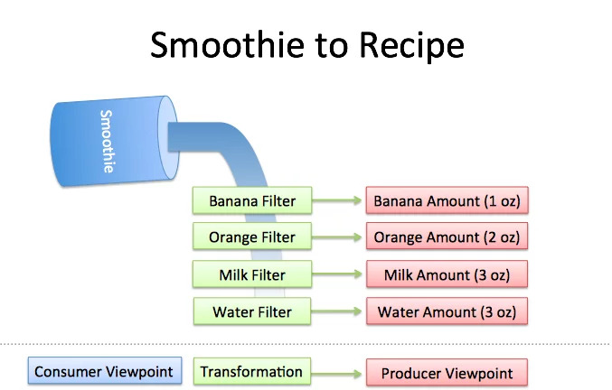
Here is a nice metaphor from Better Explained to illustrate the key idea of the Fourier Transform. In short, the Fourier Transform changes our perspective from consumer to producer, turning What do I have? into How was it made?
Now let’s talk about sine and cosine functions and how they can make waves.
The sine and the cosine functions can be depicted as the path of a point traveling around a circle at a constant speed.
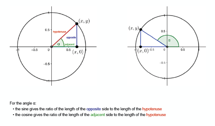
As you moved around the circle, the sine started at 0 and increased steadily until it reached a maximum of 1 when you were on top of the circle. As you kept moving it then dropped to 0 again in a symmetrical fashion, before reaching a minimum of -1, and finally coming back up again to 0. This creates a wave pattern.
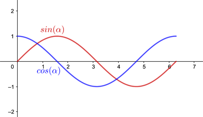
There are two important aspects of waves, which are their wavelength and amplitude. Wavelength (λ) is the distance between successive peaks. Amplitude, or intensity, is the height of each of those peaks.

We can combine two or more waves to make a new one. When multiple waves are added together, depending on the overlapping waves’ alignment of peaks and troughs, they might add up (constructive interference), or they can partially or entirely cancel each other (destructive interference).
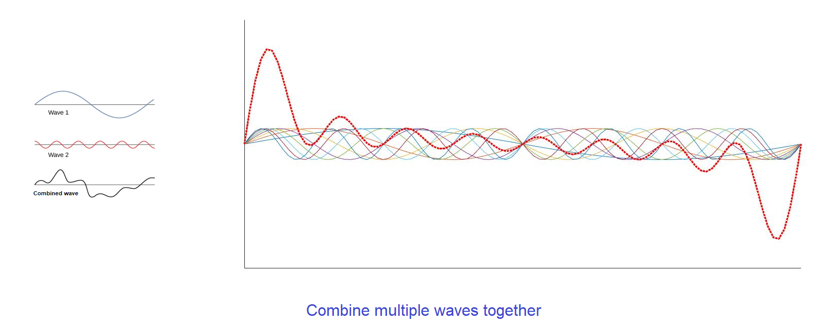
One question is, if we have a combined wave, can we split them into separate sinusoids? Well, we can, with the help of the Fourier Transform. The Fourier Transform allows us to take the combined wave, and get each sine wave back out. With that, we can view the signals in a different domain, inside which several difficult problems become very simple to analyze and process.
That's a long introduction, now let’s see the Fourier Transform in action in the world of JPEG.
Discrete Cosine Transform in JPEG
The Discrete Cosine Transform (DCT) is based on the Fourier Transform: it transforms a signal from the spatial domain to the frequency domain. The DCT is easier to compute and only involves real numbers (instead of complex values in the basic Fourier transform function).
First, the image is divided into 8x8 blocks of pixels. The DCT is then applied to each of those blocks. In the case where there are not enough pixels in a row or column to complete a full 8x8 block, some padding will be added.
Do you remember from the last part that we can combine multiple waves to make a new one? The same principles apply here: any 8x8 pixel block can be represented as a combination of component waves. More specifically, there are a total of 64 different cosine values needed to produce any of those blocks.
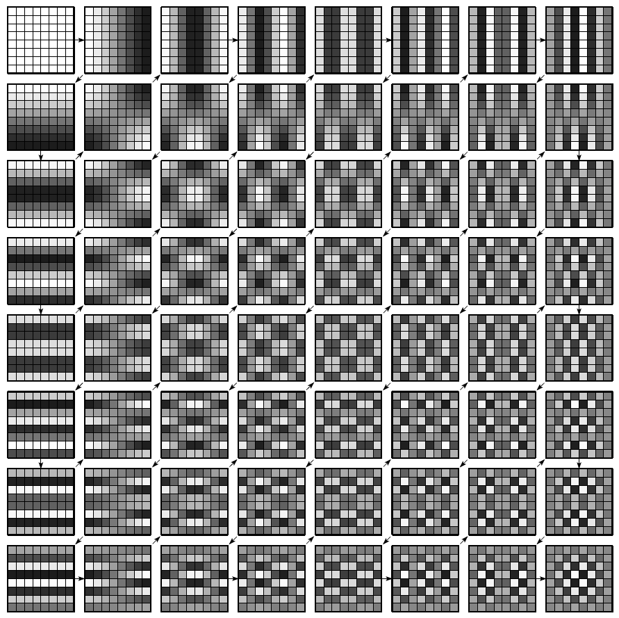
Any 8×8 block of pixels can be created by combining all of the above cosine values. Each of these values has a different contribution to the whole. Their contribution is weighted and represented as the number called coefficients.
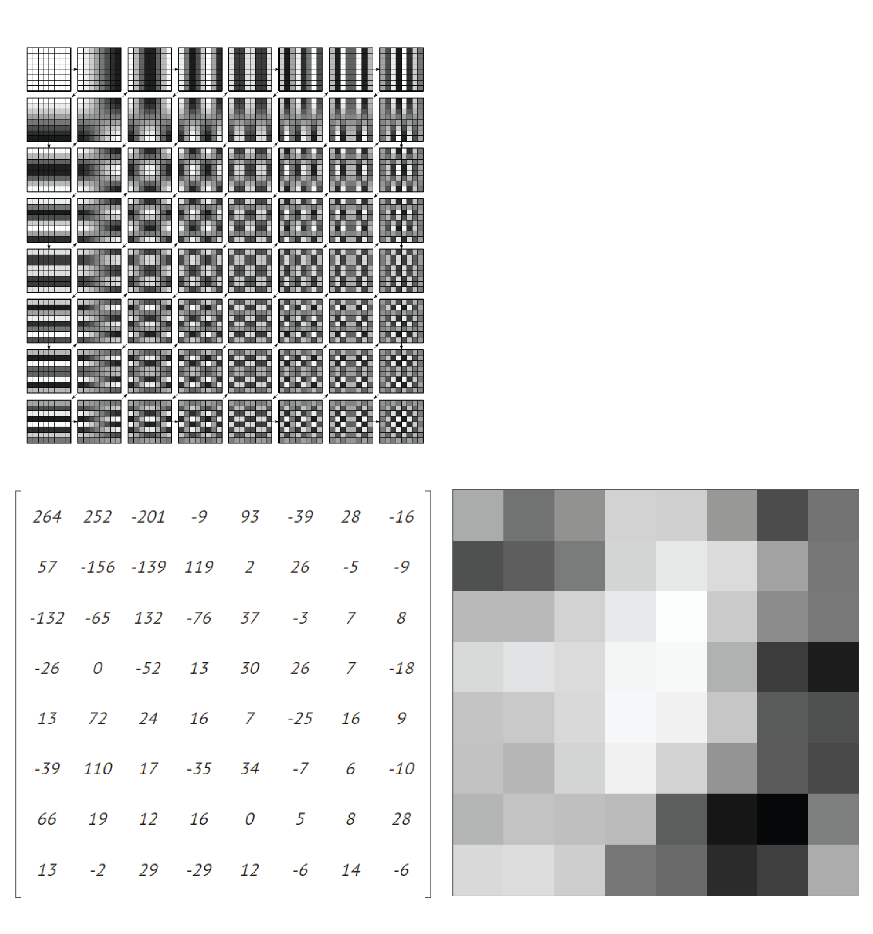
There are 64 coefficients displayed as the 8x8 matrix. The top left element in the matrix is called DC (direct current), and the other 63 is called AC (alternating current). The DC coefficient represents the average color of the 8x8 region. The 63 AC coefficients represent color change across the block.
Here is the equation to calculate those coefficients:
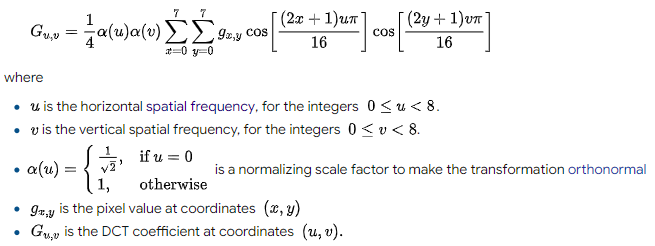
You can read more about the math on the wiki page.
With the DCT, we have a 2-D array representing the spatial frequency information of the original block. The upper-left elements of the matrix have lower frequencies, while the lower-right elements have higher frequencies.
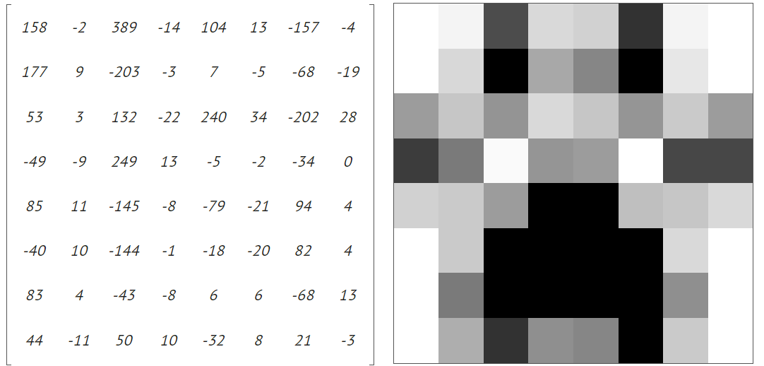
As we have discussed, the human visual system is less perceptive to errors in high-frequency spacial content, so we can discard the information there (elements near the bottom-right of the matrix). Most of the original information can be reconstructed from the lower frequency coefficients (the ones closer to the top-left).
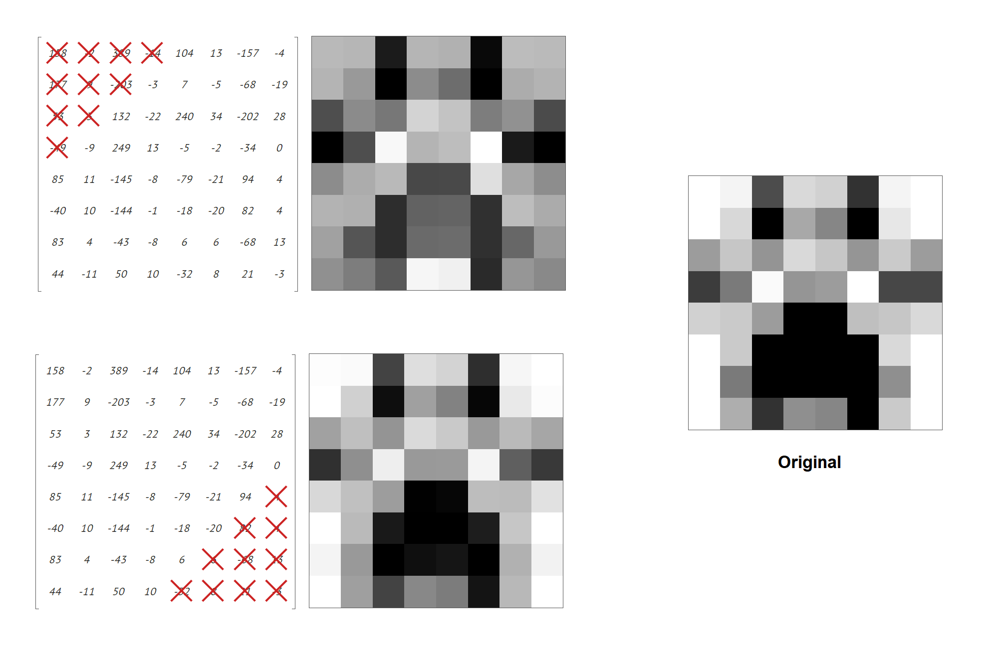
In the example above, removing the bottom coefficients is not affecting the image that much compares to removing the top coefficients.
Notes that by itself, applying the DCT to a block of color samples doesn't result in any compression. We just turned 64 color values into another 64 values (coefficients), no information is lost at this stage. This phase is a preparation for the next step, quantization, where we throw away the less significant data.
Quantization
Given the result from the DCT step, we can discard high-frequency details and preserve low-frequency information quite easily. We do this by dividing the DCT coefficient by the predefined quantization table and then rounding to the nearest integer.
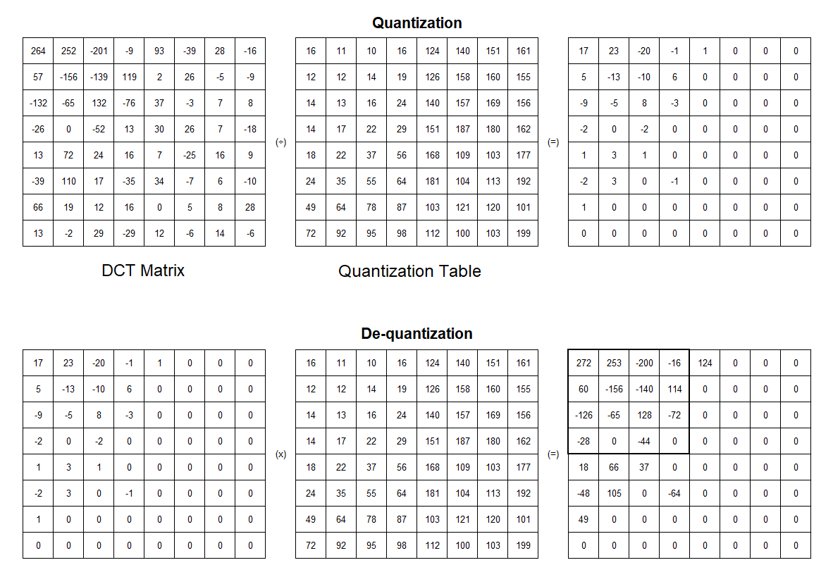
Since the goal is to remove most of the coefficients in the bottom right of the DCT matrix, the quantization table has a larger value at the bottom right. A large divisor in the table will lead to more zeros values in the result. The lower the quality setting, the greater the divisor, and the more information is thrown away. In other words, the quantization table is responsible for the quality of the JPEG image. This quantization table might vary between different digital cameras and software packages. The quantization tables are put into the header of JPEG files, so we can reconstruct the image later.
In the de-quantization stage, the quantization result we have before is multiplied with the same quantization table to get the original data. As you can see, the result after de-quantizing is not the same as the original one. Here is why JPEG compression is a lossy algorithm. Some data is a permanent loss, but most of the key information is retained.
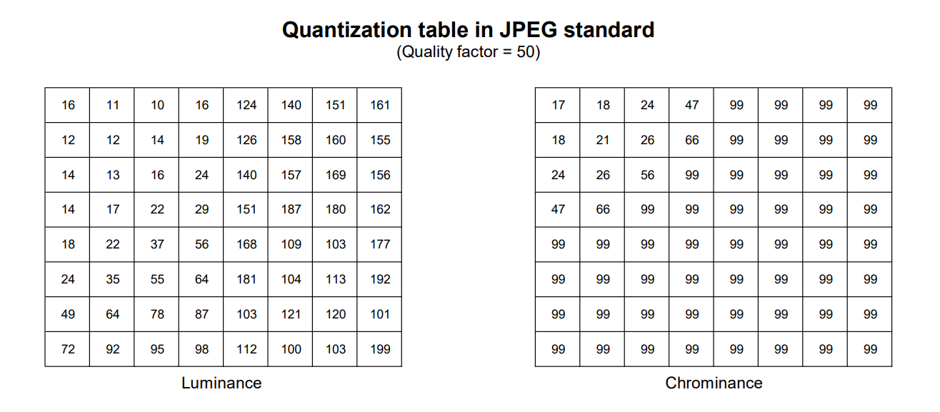
In the Chroma subsampling step, we know that the luminance is more important than the chrominance. As a result, we can remove more of the color information than luminance. Therefore, the DCT and quantization are applied for each channel separately. The JPEG standard includes two examples of quantization tables, one for the luminance channel (Y) and one for chrominance channels (Cb and Cr).
After quantization, many high-frequency components get rounded to zero, while others are transformed into much smaller values. In the final step, we will find a way to store those data effectively.
Encoding
In this last stage, several methods are used together to store the data efficiently. All of these are lossless compression (no information is lost). After the previous steps, we now have 64 coefficients that need to be stored for each block. Usually, the DC coefficients are much bigger than the others, while the AC coefficients are mostly zero after quantization. Therefore, we will treat the DC coefficients and the AC separately.
Differential Pulse Code Modulation for DC components
The Differential Pulse Code Modulation (DPCM) encodes the difference between the current DC and the previous DC.
For example, if the DC coefficients for the first 5 image blocks are 150, 155, 149, 152, 144, then the DPCM would produce 150, 5, -6, 3, -8.
We use this technique because of these observations:
The adjacent 8x8 blocks in the image have a high degree of correlation, so the DC components are often close to the previous values.
Calculating the difference from the previous DC produces a very small number that can be stored in fewer bits.
Each DPCM is then coded by the form (SIZE, AMPLITUDE), where SIZE indicates how many bits are needed for representing the coefficient, and AMPLITUDE contains the actual bits.
SIZE is Huffman coded since smaller SIZE occurs much more often. We will discuss the Huffman encoding algorithm in the latter part of this article. Basically, with the Huffman algorithm, we can create an efficient encoding table if the input data has lots of similar values. Based on this table, the data is encoded with the less bitstring as possible.
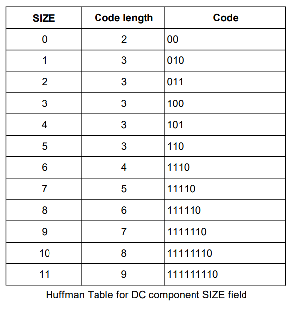
AMPLITUDE is not Huffman coded because its value can change widely. The code for AMPLITUDE is derived from the following table:
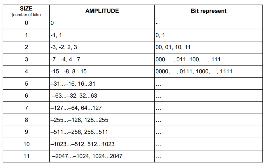
These tables are defined in the JPEG standard and specification.
For example, the value -8 will be coded as 101 0111:
0111: The value for representing -8 (see the table for AMPLITUDE)
101: We need 4 bits to represent -8. The corresponding code from the Huffman table (see the table for SIZE) for 4 is 101
Entropy encoding for AC components
After quantization, many small coefficient values toward the bottom right of the matrix become zeroes. Then the matrix is reordered from the top-left corner into a 64-element vector in a zigzag pattern. Using this method, the more important coefficients appear earlier on in the series, while the less important ones (mostly zeros) appear later on.
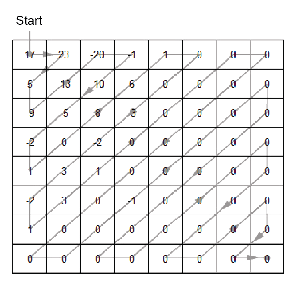
In the example above, if we order the coefficients in a zigzag pattern, we get the following string:
17 23 5 -9 -13 -20 -1 -10 -5 -2 1 0 8 6 1 0 0 -3 -2 3 -2 1 3 1 0 0 0 0 0 0 0 0 0 0 0 0 0 0 -1 0 0 0 0 0 0 0 0 0 0 0 0 0 0 0 0 0 0 0 0 0 0 0 0 0
Notices that the first value in the string (17) is the DC value, and it has been handled separately, so we don’t encode it here. We only compress the remaining 63 values.
That string has lots of zeros number in it, so one simple way is to encode the zeroes with the number of its occurrences in the sequence. So our string will become something like this:
{ 23, 5, -9, -13, -20, -1, -10, -5, -2, 1, 0 [x1], 8, 6, 1, 0 [x2], -3, -2, 3, -2, 1, 3, 1, 0 [x14], -1, 0 [x25] }
The run-length encoding method in JPEG has the same idea but with a little difference. It stores the triplet in the following format:
(RUNLENGTH_ZEROS/SIZE)(AMPLITUDE)
Where:
RUNLENGTH_ZEROS: the number of zeros that come before the current value, range from 0 to 15.
SIZE: the number of bits required to represent the current value, with range [0-A].
AMPLITUDE: the actual bit-representation of the current value.
When the number of zeros exceeds 15 before reaching another non-zero AC coefficient, we use a special code (15/0)(0). Another special value (0, 0) indicates the end of blocks, marking that all value remaining is all 0.
The (RUNLENGTH_ZEROS/SIZE) pairs and the AMPLITUDE will be encoded by using the following tables (they share some similarities to the table we have used in the DPCM step):

(Again, the full table can be found in the JPEG standard and specification)
So with the prior example string, we have:
23 5 -9 -13 -20 -1 -10 -5 -2 1 0 8 6 1 0 0 -3 -2 3 -2 1 3 1 0 0 0 0 0 0 0 0 0 0 0 0 0 0 -1 0 0 0 0 0 0 0 0 0 0 0 0 0 0 0 0 0 0 0 0 0 0 0 0 0
ⓘ The first value (23) is represented as follows: 23 → (0/5) 23 → 11010 01000
No zero comes before it, and 23 needs 5 bits to represent, refer to the table on the right.
11010: the code for (0/5), refer to the table on the left.
01000: the code for 23, refer to the table on the right.
ⓘ The -3 value in the example string appeared after 2 zeros, so it is encoded as (2/2) -3 → 11111001 00
11111001: 8 bits code for (2/2) from the left table.
00: representation of -3 from the right table.
ⓘ The last sequence of zeros is called the end of blocks (EOB) and is encoded as (0,0) → 1010
Huffman encoding
We have been using the Huffman table to encode both the DC and AC values, but we haven’t discussed where that table came from. The Huffman coding algorithm is pretty simple, but powerful and widely used in the compression process.
Overview
Let’s say we have some data that need to compress, take my name “MINH HNN” for example.
There are a total of 4 unique characters in that string, “M”, “I”, “N”, and “H”. We are going to encode each character using a unique string of bits. We can pick any series of bits we like to represent each character, as long as we can decode it to get the original.
Here is a simple data representation, using two bits for each character:
M    →    00
I    →    01
N    →    10
H    →    11
So the string “MINHHNN” can be compressed as 00011011111010 (16 bits), which is more efficient than store as an ASCII or UTF-8 value. But we can do better than this. In the example, the character “N” and ”H” appears more than the others. If we give a shorter code to "M" and “H”, then we will be using less space.
M    →    011
I    →    010
N    →    1
H    →    00
In this way, the compressed bitstring 0110101000011 is only 13 bits.
The only restriction when choosing the represented bitstrings with different lengths is that they must be prefix-free, none of them can be a prefix of another. Let’s say we choose "0011" to represent the letter “M”, "00" to represent "I", and "11" for "N". When decoding the text, if we find "0011", how are we supposed to know whether that was originally a letter "M", or the two letters "I" and "N"?
Another question that comes to mind is how can we find the most optimal code to represent these characters.
Fortunately, the Huffman code can help us with these problems. In the context of Huffman coding, the values that need to compress are called "symbols". Huffman’s algorithm encodes information using variable-length strings to represent symbols depending on how frequently they appear. The idea here is the symbols that are used more frequently should be shorter, while symbols that appear more rarely can be longer. This way, the number of bits it takes to encode a given message will be shorter, on average, than if a fixed-length code was used. The Huffman codes are always prefix-free.
Implementation of Huffman coding
Before jumping to the implementation of the Huffman coding, it’s actually easier to visualize by looking at the result of the algorithm. The result of Huffman coding is expressed as a “tree” structure:
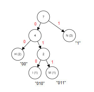
Using this tree, the number of bits used to encode each symbol equals the number of links between its tree node and the root node (the top). Remember that we want the most occurrences symbol to have the shortest code. We keep track of each leaf node with a “weight”, which is simply the number of times its symbol appears in the input data. The leaf nodes that have a bigger weight will be closer to the root, thus having shorter bitstrings.
Now we have some sense of the result, let’s start building this tree from scratch, using the same string example "MINHHNN".
The first step is to count how many times each symbol occurs (sometimes called frequency or probability).
M    →     1
I     →    1
N     →    3
H    →    2
The goal is to build a tree in which the most occurrences symbol is at the top, and the least common symbol is at the bottom. Here we tackle the problem with the bottom-up approach.
“M” and “I” have the least appearances, so these two will be at the bottom.

Next, we continue finding the two symbols that have the smallest counts. Since we have combined the two characters “M” and “I”, we use the total count of these two.
(M, I)    →     2
N         →    3
H        →    2
The same step is repeated, choosing the two smallest values to make a new branch. Right now, "(M, I)" and "H" have the smallest counts so we combine them.
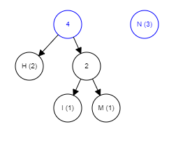
The rest of the algorithm is pretty straightforward, just keep picking the two lowest-weighted subtrees and join them together until there is only one tree remaining, it is the completed tree.
Below is the GIF that summarizes the whole process, you can try it yourself here.
The Huffman coding is a lossless algorithm that works best when the input contains symbols that are way more likely to appear than the others. JPEG compression uses this method because there are lots of duplicate values after the quantization stage.
There are some differences between the Huffman coding used in JPEG and the basic algorithm described above.
The first difference is that the JPEG Huffman tables never use bitstrings which are composed of only 1's, i.e. "111" or “11111”. Because the sections of Huffman-coded data in a JPEG file must always occupy a whole number of 8-bit bytes, if there are some extra bits left to fill in the last byte, "1" bits are used as padding. To avoid confusion when decoding, the bitstrings composed of only 1's are left out.
The second difference is that JPEG Huffman codes are always canonical. That means when the bitstrings are read as binary numbers, shorter bitstrings are always smaller numbers. For example, such a code could not use both "000" (number 0 in decimal) and "10" (number 2 in decimal), since the former bitstring is longer, but is a smaller binary number. This helps the JPEG files smaller and faster to decode.
You can read more about the JPEG Huffman coding at Alexdowad’s blog.
Summary
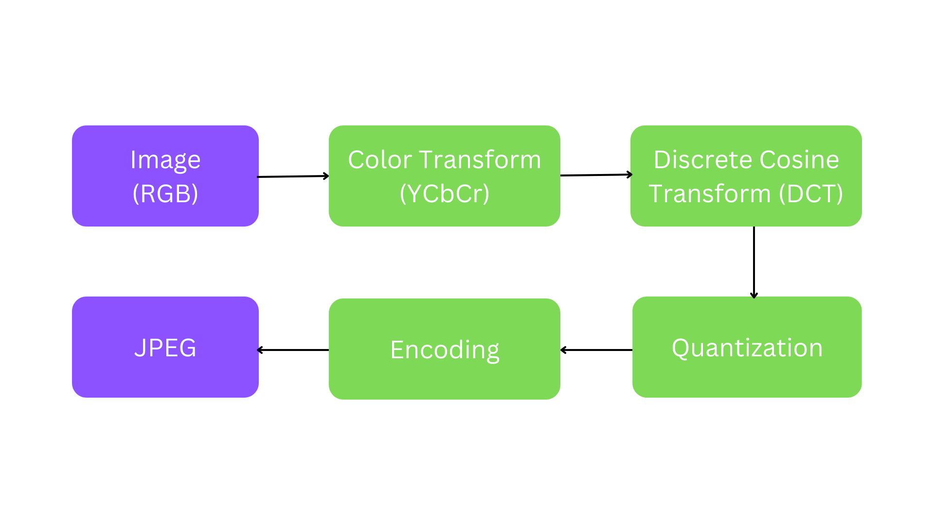
Below is the recap of the JPEG compression process.
JPEG images have been existing since the early 1990s and still dominate the world today. They can store a lot of data in a small file size, which makes them ideal for everything from digital photos to web graphics.
On the flip side, when dealing with very heavily compressed images, the quality will suffer. Some photographers don’t like shooting in JPEGs because they want to keep all the image detail for post-processing or printing. But this file format is still very much a mainstream favorite.
The next generation of JPEG, called JPEG XL, has been published in 2019. It is designed to outperform existing formats and thus become the universal replacement. JPEG XL can meet the needs of both image delivery on the web and professional photography. It further includes features such as animation, alpha channels, layers, thumbnails, and lossless and progressive coding to support a wide range of use cases including e-commerce, social media, and cloud storage. JPEG XL, like most other JPEG standards, is a multipart specification. Some of the parts are currently under development, so let’s wait to see how it becomes in the future.
That’s all for today, hope you enjoyed this post. See you later.
References:
An Interactive Guide To The Fourier Transform
The Ultimate Guide to JPEG Including JPEG Compression & Encoding
JPEG Series, Alex Dowad Computes
The Unreasonable Effectiveness of JPEG: A Signal Processing Approach


